This quick start guide provides a very brief introduction to the LaharFlow web user interface.
LaharFlow works best on recent web browsers. In particular, we do not recommend the use of versions of Internet Explorer earlier than version 8, versions of Firefox prior to 4.0, or versions of Chrome prior to 6.0. If you have any difficulties running LaharFlow, please feel free to contact laharflow-info@bristol.ac.uk.
After logging into LaharFlow, you arrive at the main LaharFlow page where settings for the calculation are specified, the calculation is started and the results are displayed and can be exported.
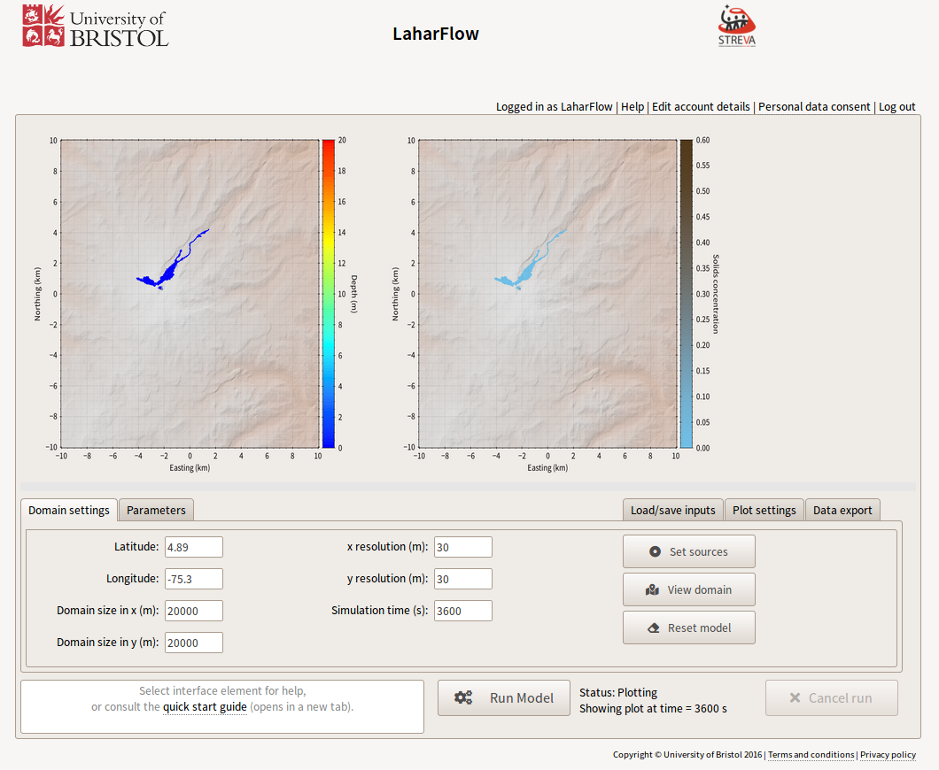
The main screen is composed of an upper panel, where plots of the LaharFlow calculation are displayed, and a lower panel containing a series of tabs to take user input and control the display and export of model output. If you are logging in for the first time, you will see that the upper plots panel is empty. If you have a completed calculation, or have logged in while a calculation is running, then you will see graphical results in the upper panel.
Settings for the LaharFlow calculation are supplied through the lower input panels:
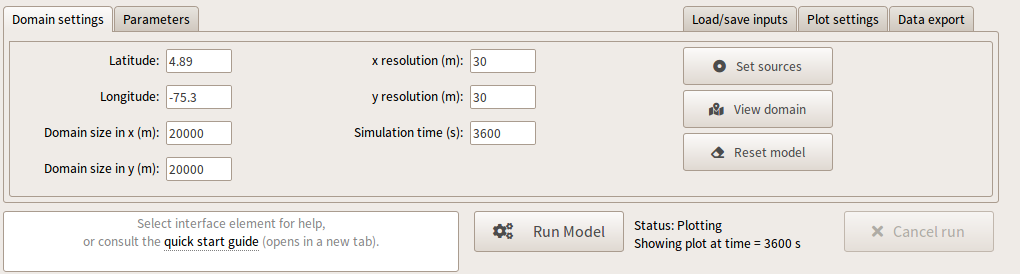
When a input box is selected, a short description of the parameter is displayed in the lower-left of the page, and, for numeric parameters, the maximum and minimum values permitted are displayed to the right of the parameter input box.
The location of the calculation and computational domain settings for LaharFlow are specified in the Domain settings tab.
Parameter values for the calculation are set in the Parameters tab.
On the right hand side, the Plot settings tab controls the plots that are displayed in the upper panel, and the output from LaharFlow can be exported using the options in the Data export tab. Details of these tabs are given in the following sections.
The LaharFlow calculation takes place on a digital topographic map, so the location of the simulation is essential. The centre of the domain, the domain size and the numerical resolution of the calculation are all specified in the Domain settings tab. The time of the flow simulation is also specified in this tab.
When the domain settings are specified, the flow domain topography can be viewed by clicking on the button. With the domain settings on first log-in, the view domain shows:
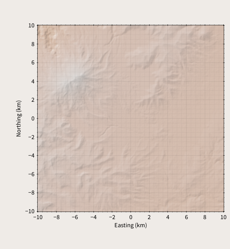
The Domain settings tab also has buttons for setting sources, described below.
Lahar material is added to the calculation through the buttons in the Domain settings tab. There are two types of sources: cap sources, where all the material is released at one time; and flux sources, where the material is released over time. Further details of these types of sources is available.
Clicking the button opens a new input screen:
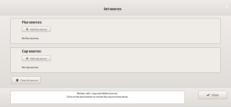
The "Set Sources" screen allows for cap sources and flux sources to be added, edited, copied, reviewed and deleted. On the first login, the "Set Sources" list is empty. On subsequent logins, the "Set Sources" list will display the sources that have been added in the current simulation, if any.
The "Set Sources" screen is closed by clicking on the button. Note the button is only active if there are no errors in the sources that have been added and no duplicate sources.
Clicking the button on the "Set Sources" screen opens a new input screen:
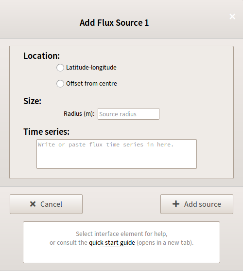
On this input screen the attributes of a flux source are set.
The location of the flux source can be given either as a latitude-longitude coordinate, or as a offset distance from the centre of the domain. Selecting the form of the location opens input boxes for entering the numerical values.
The size of the flux source is determined by specifying the 'Radius'.
The volumetric flux of material and the solids concentration is input as a time series in the 'Time series' text box. The time series must be entered as comma separated values in three rows. The first row is the time, the second row is the volume flux, and the third row is the solids concentration. There must be the same number of data points in each row.
The flux source is added to the simulation by clicking the button, once all the inputs are set. The list of flux sources on the "Set Sources" screen will be updated to display the details of the flux source.
Clicking on clears the inputs and closes the flux source input screen.
Clicking the button on the "Set Sources" screen opens a new input screen:
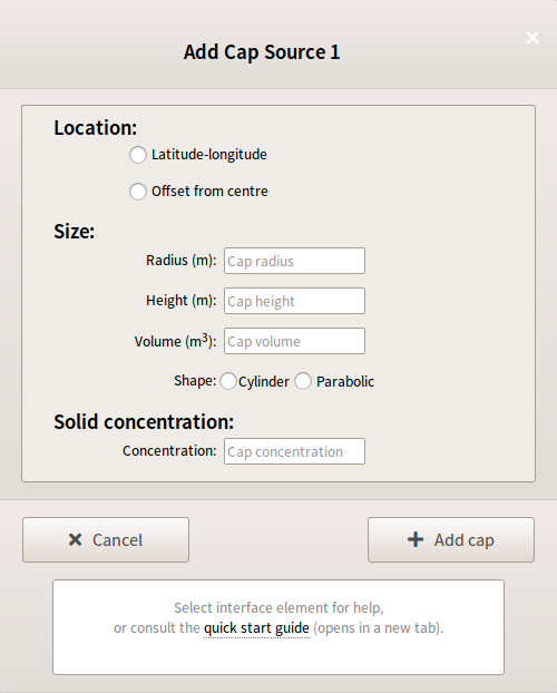
Here the attributes of the cap source are set.
The location of the cap source can be given either as a latitude-longitude coordinate, or as a offset distance from the centre of the domain. Selecting the form of the location opens input boxes for entering the numerical values.
The size of the cap is determined by specifying two out of the 'Radius', 'Height' and 'Volume'.
The shape of the cap must also be set, either as a 'Cylinder' or a 'Parabolic' cap.
Finally, the 'Concentration' of solids in the cap of material must be specified. Further information on cap sources is available.
The cap source is added to the calcution by clicking the button, once all the inputs are set. The list of cap sources on the "Set Sources" screen will be updated to display the details of the cap source.
Clicking on clears the inputs and closes the cap source input screen.
Once at least one source has been added, the "Set Sources" screen displays lists of the flux and cap sources that have been added to LaharFlow.
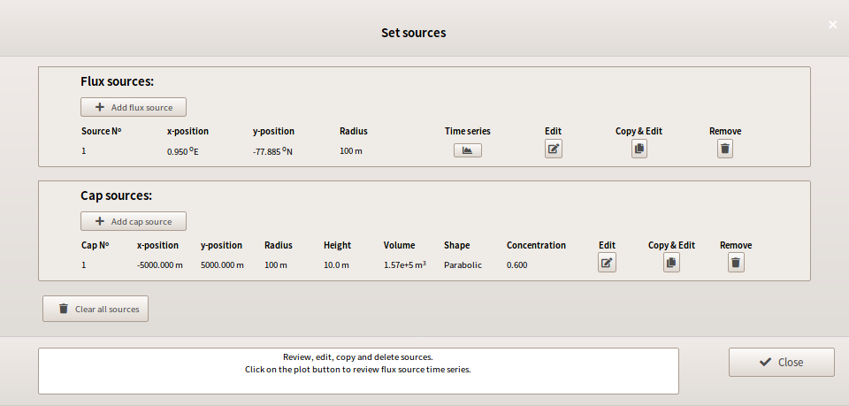
In the example above, two sources have been added: one cap source and one flux source.
The cap source was positioned as an offset from the centre of the domain. The radius and height were specified and the corresponding volume calculated. The shape was set as 'Parabolic' and a solids concentration of 0.6 (60%).
The flux source was positioned using latitude-longitude coordinates. A radius and time series were specified. The 'hydrograph' input as the time series can be viewed by clicking the 'Time series' button:
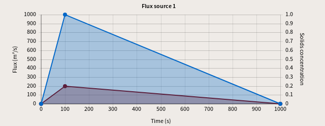
Here a simple time series was used, with three data points for the time, flux and concentration.
The blue curve shows the volumetric flux time series. The red curve shows the solids concentration time series.
Clicking on the 'Time series' button a second time will close the time series plot.
Sources that have been added to LaharFlow can be edited on the "Set Sources" screen by clicking on the 'Edit' button in the lists of sources. This will open a screen which allows the source attributes to the modified.
New sources can be added by copying and editing existing sources on the "Set Sources" screen by clicking on the 'Copy & Edit' in the lists of sources. This will open a screen with the attributes of the copied source which can be modified.
Note, identical sources are not permitted.
Sources in the lists on the "Set Sources" screen can be removed by clicking on the 'Remove' in the lists of sources. The source is removed immediately.
All the sources in the lists can be cleared by clicking the button. The sources are removed immediately.
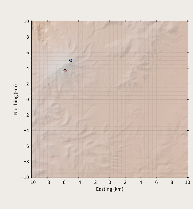
After adding at least one source and closing the "Set Sources" screen, clicking on will display the topography of the flow domain together with markers displaying the location of the sources.
When at least one source has been added, the LaharFlow calculation can be started by clicking the button.
The status will change:

and will indicate the progress of the calculation.
As the calculation progresses, plots are displayed to illustrate the results.
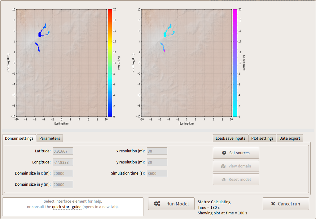
The calculation can be cancelled by clicking the button.
In the example above, two diagnostic plots are shown. Further information about the plots is available.
The Plot settings tab allows the plots displayed to be controlled.
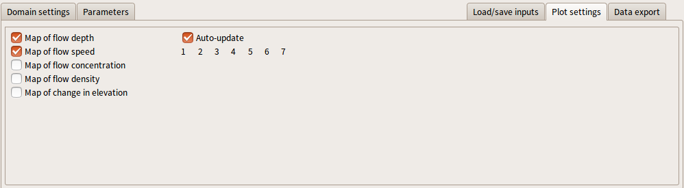
On the left-hand side of the tab there is a selectable list of the plots that can be displayed:
- Map of the flow depth
- Map of the flow speed
- Map of the flow concentration
- Map of the flow density
- Map of the change in elevation of the topography due to erosion and deposition
The table shows the plots that are available to view. The table updates as the calculation progresses, producing 100 image sets at 100 time instances. In the example above, 7 of the image sets have been produced.
If the 'Auto-update' checkbox is selected, as in the example above, then new image sets are displayed when they become available, updating the plot display panel. If unselected, the table will update but the plot display panel will show the chosen or last displayed plots.
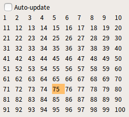
The image set labels in the updating table are selectable and on selection the plot display panel will show the corresponding images. In the example below, the image set 75 is selected. Note, when selecting image sets it is useful to switch-off 'Auto-update'.
More information about viewing and interpreting the plots is available.
Results of the model can be exported from the Data export tab.
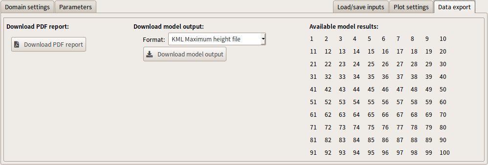
There is again an updating table, on the right-hand side of the tab, showing the available model data sets. The table updates as the calculation progresses, showing which of 100 data sets at 100 time instances are available to be downloaded. In the example above, the calculation has completed, so all 100 result data sets are available.
In the centre of the Data export tab there is a drop-down menu allowing type of data export to be selected.
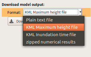
There are four download types that can be selected:
- Plain text file
- KML Maximum height file
- KML Inundation time file
- zipped numerical results
If 'Plain text file' is selected as the data type, then a data set (i.e. a time instance in the calculation) must be selected from the table on the right.
Once the data type (and data set, if required) is selected, the data can be downloaded by clicking on the button.
Note data download can be slow over wireless or slow web connections, particularly if 'zipped numerical results' are downloaded.
The button produces and downloads a PDF document that reports the domain settings and parameter values used in the calculation and includes some plots.
The Parameters tab allows parameter values in the LaharFlow model to be changed.
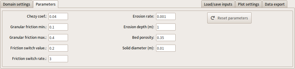
The left-hand column has parameters related to the drag formulation of LaharFlow. The right-hand column has parameters related to the morphodynamics of erosion and deposition.
More information about the parameter is available.
The Load/save inputs tab allows the settings of the LaharFlow model to be saved and subsequently reloaded.
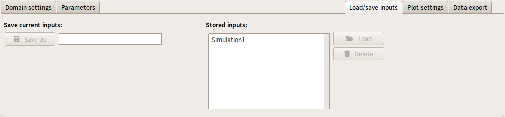
The current inputs to LaharFlow, including the domain settings, sources and parameters, can be saved. Note, model results and images are not saved.
A name for the input set must be specified, using the 'Save current entry' box.
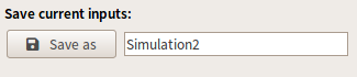
Clicking on the button saves the inputs, which are added to the list of 'Stored inputs'.
Input sets in the 'Stored inputs' list can be loaded by selecting the input set name and clicking on the button.
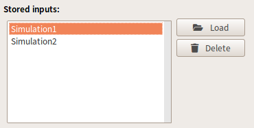
Clicking on the button will delete the selected input set.